ML Note#2:Linear Models(2)
ML系列学习笔记基于吴恩达教授的斯坦福CS229 2018课程📒
本文扩展了线性回归模型:引入局部权重回归以及第一个分类模型——逻辑斯特回归;证明为什么使用最小平方误差作为优化目标;介绍一种新的参数优化方法——牛顿法。
Locally Weighted Linear Regression
局部权重回归,一种直接实现非线性回归的模型。
- Ahead: two types learning algorithms
- parametric: fit fixed set of parameters to data.
- *non parametric: the amount of data/parameters need to keep growing (linearly) with the size of data.
- Crucial Idea: to evaluate \(h\) at a certain input \(x\), consider more about the data with inputs \(x\). (consider neighbors more)
Target优化目标
Fitting \(\theta\) to minimize: \[ \sum^m_{i=1}w^{(i)}(y^{(i)}-\theta^Tx^{(i)})^2 \] where \(w^{(i)}\) is the weight: \[ w^{(i)}=\mathrm{exp}(-\frac{(x^{(i)}-x)^2}{2\tau^2}) \]
- \(\tau\): a hyperparameter to control the weight. (may leading to overfitting or underfitting)
Least Squares 最小平方误差?
为什么通过最小平方误差选择参数?
Firstly, assume \[ y^{(i)}=\theta^Tx^{(i)}+\varepsilon^{(i)} \] where \(\varepsilon\) is the "error", an unmodeled effect also referred to as the random noise.
Assume the \(\varepsilon\) follows a Normal distribution. (default) \[ \varepsilon\sim N(0,\sigma^2) \]
\[ P(\varepsilon)=\frac{1}{\sqrt{2\pi}\sigma}\mathrm{exp}(-\frac{\varepsilon^2}{2\sigma^2}) \]
Then \[ \begin{aligned} P(y^{(i)}\mid x^{(i)}; \theta) & =\frac{1}{\sqrt{2\pi}\sigma}\mathrm{exp}(-\frac{(y^{(i)}-\theta^Tx^{(i)})^2}{2\sigma^2})\\\\\\\\ & \sim N(\theta^Tx^{(i)}, \sigma^2) \end{aligned} \] The likelihood of \(\theta\) \[ \begin{aligned} L(\theta) & =P(y\mid x;\theta)\\\\ & =\prod^m_{i=1}P(y^{(i)}\mid x^{(i)};\theta)\\\\ & =\prod^m_{i=1}\frac{1}{\sqrt{2\pi}\sigma}\mathrm{exp}(-\frac{(y^{(i)}-\theta^Tx^{(i)})^2}{2\sigma^2}) \end{aligned} \] Transfer to log-likelihood \[ \begin{aligned} l(\theta) &=\mathrm{log}L(\theta)\\ &=m\mathrm{log}\frac{1}{\sqrt{2\pi}\sigma}+\sum^m_{i=1}-\frac{(y^{(i)}-\theta^Tx^{(i)})^2}{2\sigma^2}\\ \end{aligned} \] Choose \(\theta\) by the maximum likelihood estimation (MLE)
i.e. minimize: \[ \frac{1}{2}\sum^m_{i=1}(y^{(i)}-\theta^Tx^{(i)})^2 \] which is the cost function \(J(\theta)\) before.
Logistic Regression逻辑斯特回归
逻辑斯特回归,用回归思想解决(二)分类问题。
Ahead前言
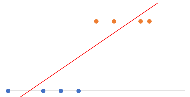
why not linear regression?
seems it works too. (using a decision value to discriminate two categories)

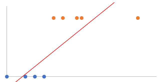
but the regression line can be easily impacted by a remote point.
e.g.

the orange point on the right side heavily influences the decision line.
Idea想法
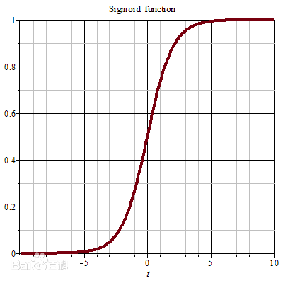
want a hypothesis: \(h_\theta(x)\in[0,
1]\) (probability of the positive class) \[
h_\theta(x)=g(\theta^Tx)=\frac{1}{1+e^{-\theta^Tx}}
\] where \(g\) is also referred
to as "sigmoid" or "logistic" function. (setting a cap for the influence
of the remote point) \[
g(z)=\frac{1}{1+e^{-z}}
\]

so that \[ P(y\mid x;\theta)=h_\theta(x)^y(1-h_\theta(x))^{(1-y)} \]
Likelihood似然函数
\[ \begin{aligned} L(\theta) &=P(y\mid x;\theta)\\\\ &=\prod^m_{i=1}P(y^{(i)}\mid x^{(i)};\theta)\\\\ &=\prod^m_{i=1}h_\theta(x^{(i)})^{y^{(i)}}(1-h_\theta(x^{(i)}))^{(1-{y^{(i)}})} \end{aligned} \] transfer to log likelihood \(l\) \[ \begin{aligned} l(\theta) &=\mathrm{log}L(\theta)\\\\ &=\sum^m_{i=1}[y^{(i)}\mathrm{log}h_\theta(x^{(i)})+(1-y^{(i)})\mathrm{log}(1-h_\theta(x^{(i)}))] \end{aligned} \]
Update参数更新
batch gradient ascent \[ \begin{aligned} \theta_j &:=\theta_j+\alpha\frac{\partial}{\partial \theta_j}l(\theta)\\\\ &=\theta_j+\alpha\sum^m_{i=1}(y^{(i)}-h_\theta(x^{(i)}))x^{(i)}_j \end{aligned} \] maximizing the likelihood (uphill).
*same to the one for the linear regression (explain later)
Newton's Method牛顿法
牛顿迭代法,更快的参数优化方法。
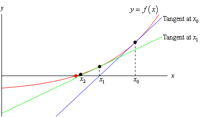
given a function \(f(\theta)\), want to find a \(\theta\)
s.t. \(f(\theta)=0\)
- set a random \(\theta_0\)
- (repeat) calculate the tangent, update \(\theta\) with the value where the tangent cross the horizontal axis.
 \[
\theta^{(t+1)}:=\theta^{t}-\frac{f(\theta^t)}{f'(\theta^t)}
\]
Apply to ML 应用
regard the gradient of log likelihood \(l(\theta)\) or the cost function as \(f\). \[ \theta^{(t+1)}:=\theta^t-\frac{l'(\theta^t)}{l''(\theta^t)} \] when \(\theta\) is a vector \[ \theta^{(t+1)}:=\theta^t-H^{-1}\nabla_\theta l(\theta) \] where \(H\) is the Hessian matrix \[ H_{ij}=\frac{\partial^2}{\partial\theta_i\partial\theta_j} \]
Characteristic特性
- Pros: faster convergence, "quadratic convergence".
- Cons: expensive to compute the \(H\) when dim is high.
Questions问题
- How about other cost functions besides square error? (just told why we can use the least square)
Vocab词汇
- square root 平方根